Augmenting Financial Analysis with Agentic AI Workflows
Agentic AI turns your finance stack into a set of closed-loop workflows that plan, execute, and verify analysis—then hand decisions to humans with evidence. Instead of “copilots” that draft text, these agents query governed data, reconcile results, forecast with uncertainty bands, propose actions, and write back to your ARR Snowball, cash, and board packs—under tight controls.
What “agentic” means in finance
Agentic AI is software that can plan, act, and self-check toward a goal—not just chat. It orchestrates a closed-loop workflow (plan → retrieve → act → verify → handoff), running queries and models on governed data, reconciling results, and proposing or executing actions under constraints with audit trails and approvals. In short: an analyst that does the work, not just drafts it. Here are the high level steps that an agentic AI workflow would take:
- Plans the task (e.g., “explain NRR variance vs. plan”),
- Retrieves the right definitions and historical context,
- Acts by running SQL/Python on governed data and using approved tools (forecast libs, optimizers),
- Self-checks results (unit tests, reasonableness checks),
- Outputs analysis + recommendations to the target system (Power BI/Tableau, tickets),
- Asks approval when money or policy is involved.
Think of an analyst who never forgets the metric glossary, never skips reconciliation, and always attaches their SQL.
Where agentic AI adds real leverage
Here are sample agentic AI workflows—grounded in the ARR Snowball and Finance Hub patterns from this blog series—that deliver real leverage. Each use case plans the task, pulls governed data, runs forecasts/causal/optimization models, self-checks results, and writes back actionable recommendations with owners, confidence, and audit trails. Treat these as templates to pilot on top of your existing Fabric/Snowflake/Power BI stack.
1) Close Acceleration & GL Integrity
This use case runs on top of a governed Finance Hub—the daily, finance-grade pipelines outlined in our Resilient Data Pipelines for Finance. With GL, subledgers (AR/AP), billing, bank feeds, payroll, and fixed assets unified with lineage and controls, an agent can pre-close reconcile, flag mispostings and duplicate entries, propose reclasses with evidence, and attach audit-ready notes—shrinking time-to-close while raising confidence in reported numbers.
- Agent: Reconciliation & Anomaly Agent
- Does: auto-matches subledgers to GL, flags mispostings, proposes reclasses with evidence and confidence.
- Tech: embeddings for fuzzy matching, rules + isolation forests, templated journal suggestions.
- Output: a ranked reclass queue with impact to P&L, links to underlying entries, and audit notes.
2) ARR Snowball → Probabilistic Forecast + Prescriptive Actions
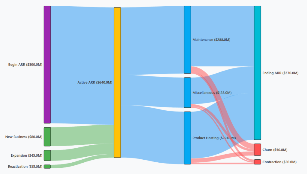
Built on the Snowball data model and definitions from ARR Snowball: Proving Revenue Durability, this workflow ingests pipeline, renewals, usage, and billing signals to produce a calibrated forward ARR curve (base/upside/downside bands). It then runs constrained optimization to select the highest-ROI save/expand plays (owners, costs, expected lift) that maximize NRR under budget and capacity, with guardrails and audit-ready lineage.
- Agent: ARR Planner
- Does: converts pipeline/renewals/usage into a probabilistic forward ARR curve; recommends the portfolio of save/expand actions that maximizes NRR under budget/capacity.
- Tech: hierarchical time-series + renewal/expansion propensity; mixed-integer optimization for action selection.
- Output: Base/Upside/Downside bands, top drivers of variance, and a monthly action schedule (owners, due dates).
3) Cash Flow with Contract Awareness
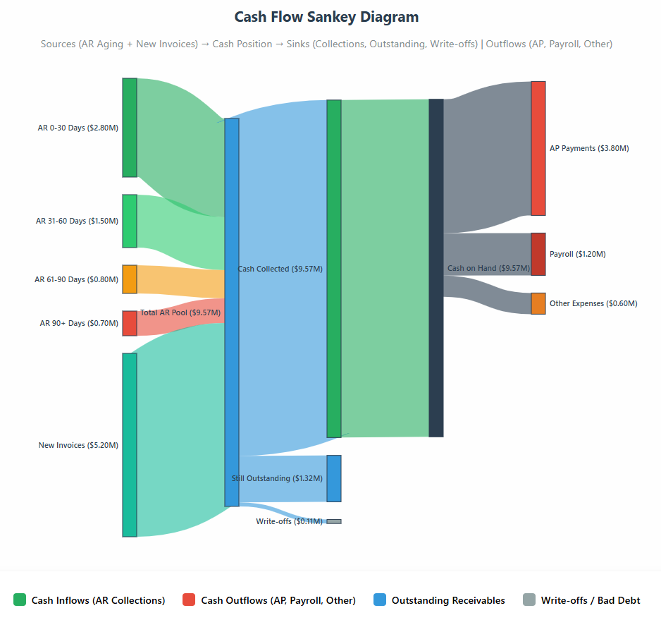
Building on the Cash-Flow Snowball outlined in Extending Snowball to Cash & Inventory, this agent (“Cash Orchestrator”) turns contracts into cash signals: it extracts renewal and payment terms, unifies AR/AP with governed ledger data, and constructs a calendarized view of expected inflows/outflows. From there, it runs a 13-week stochastic cash simulation and proposes term mixes (early-pay incentives, cadence, invoicing options) that improve cash conversion cycle (CCC) without eroding NRR—backed by bi-objective optimization (NPV vs. CCC) and full audit trails.
- Agent: Cash Orchestrator
- Does: extracts terms from contracts, joins AR/AP, simulates collections & payment runs, and proposes term mixes (early-pay incentives, cadence) that improve CCC without hurting NRR.
- Tech: LLM extraction (renewals, uplifts), stochastic cash simulation, bi-objective optimization (NPV vs. CCC).
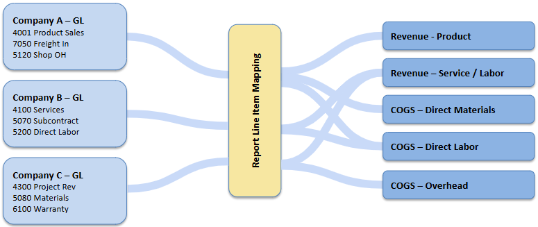
4) Cost Allocation When Detail Is Thin
Extending the approach in Cost Allocation When You Don’t Have Invoice-Level Detail, this workflow ingests GL lines, vendor metadata, PO text, and operational drivers (products, jobs, regions). An agent uses embeddings and probabilistic matching—constrained to reconcile totals back to the GL—to propose allocations with confidence scores, surface exceptions for human approval, and write back auditable adjustments. The result is consistent product/segment margins and board-ready views even when source detail is sparse.
- Agent: Allocator
- Does: maps GL lines to drivers (products, jobs, regions) using embeddings + historical patterns; produces confidence-scored allocations with human approval.
- Tech: weak supervision, constrained optimization to keep totals consistent with the GL.
5) Variance Analysis that’s Actually Causal
Built on the Snowball definitions from ARR Snowball: Proving Revenue Durability, this agent explains “why” by linking changes in NRR/GRR to causal drivers (onboarding TTV, pricing, usage) with sourced metrics and lineage.
- Agent: Root-Cause Analyst
- Does: traces “why” using causal graphs: e.g., NRR −2 pts ← onboarding TTV +9 days in SMB-Q2 cohort ← implementation staffing shortfall.
- Tech: causal discovery + do-calculus; renders a sourced narrative with links to metrics and lineage.
Reference architecture
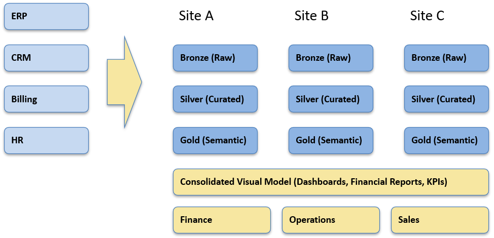
This high level reference architecture is used to run agentic AI on your existing lakehouse/warehouse without changing metric logic. It separates concerns into a governed data plane (tables, lineage), a knowledge plane (versioned metric contracts + vector store), a compute/tools plane (SQL/Python, forecasters, optimizers), orchestration (events, schedules, retries), and governance/observability (policy engine, approvals, audit, PII).
Irrespective of the underlying framework, the architecture can work through connectors for Microsoft Fabric, Snowflake, or Databricks and the workflow pattern stays the same, with outputs back to BI (Power BI/Tableau).
- Data plane: governed lakehouse/warehouse; metric contracts (GRR/NRR definitions) in a versioned glossary.
- Tooling: SQL/Python execution sandbox; forecasters (Prophet/ARIMA/Bayesian), optimizers (OR-Tools/pyomo), anomaly libs.
- Knowledge: vector store over metric dictionary, SQL lineage, policy docs (for RAG).
- Orchestration: event triggers (month-end, weekly ARR, daily cash), queue, retries, alerts.
- Governance: policy engine (who can do what), audit log of every query/action, PII redaction, secrets vault.
- UX: push to BI (ARR Sankey/forecast bands), create tickets, and draft board commentary with citations.
How it runs: the agent loop
Now that we’ve covered the use cases and architecture, this list shows the runtime lifecycle every agent follows—plan → retrieve → act → verify → propose → approve → learn—so outputs are consistent, governed, and easy to audit across ARR, cash, and close workflows.
- Plan: build a step list from the request (“Explain NRR miss in Sept”).
- Retrieve: pull metric definitions + last 12 months context.
- Act: run parameterized SQL/Python; if a forecast, produce bands + calibration stats (MAPE/WAPE).
- Verify: unit tests (sums match GL), reasonableness checks (guardrails), anomaly thresholds.
- Propose: attach SQL + charts + recommended actions, with impact estimates.
- Approve: route to owner; on approve, write back tags/notes and schedule the action.
- Learn: compare predicted vs. actual; update models monthly.
Putting it to work: example workflow map
With the loop defined, here’s how it lands in operations: a simple runbook of when each agent fires, the data/tools it uses, the outputs it produces, and the owner/KPIs who keep it honest. Use this as your starting calendar and adjust SLAs and thresholds to your portfolio.
| Workflow | Trigger | Tools & data | Primary outputs | Owner | KPIs |
|---|---|---|---|---|---|
| NRR Forecast & Action Plan | Monthly Snowball review | Usage, CRM, billing, optimizer | Forecast bands; top 10 save/expand plays | VP CS / RevOps | NRR Δ, WAPE, action adoption |
| Close Reconciliation | EOM −2 to +3 | GL, subledgers, anomaly detector | Reclass proposals, risk heatmap | Controller | Close time, reclass rate, % auto-accepted |
| Cash Horizon | Weekly | Contracts, AR/AP, scenarios | 13-wk cash projection; term mix recs | CFO | CCC, DSO/DPO, forecast error |
| Cost Allocation Assist | Monthly | GL, drivers, embeddings | Allocation file + confidence | FP&A | % manual effort saved, variance to audited |
| Variance Root Cause | On miss > threshold | Snowball, staffing, pricing/events | Causal narrative + corrective plays | FP&A / Ops | Time-to-cause, fix adoption |
A simple agent spec (YAML)
To make agents portable and auditable, define them in YAML—a compact, declarative contract that captures the agent’s goal, allowed tools/data, ordered steps (the agent loop), validations/approvals, outputs, and schedule. Checked into Git and loaded by your runner, the same spec can move from dev → stage → prod on Fabric/Snowflake/Databricks with no code changes—just configuration—while enforcing policy and producing consistent, testable results.
agent: arr_planner_v1
goal: "Produce next-12-month ARR forecast with actions to maximize NRR under constraints."
inputs:
  data:
    - table: arr_events # new, expansion, contraction, churn
    - table: usage_signals
    - table: renewals
    - table: opportunities
  glossary: metrics_v1_3 # GRR/NRR, inflow/outflow taxonomy
steps:
  - retrieve_definitions
  - build_features: [renewal_prob, expansion_rate, contraction_rate]
  - forecast_hierarchy: horizon=12, bands=[base,upside,downside]
  - optimize_actions:
      objective: maximize_net_arr
      constraints: {cs_hours<=600, discount_floor>=-15%}
  - validate: [gl_bridge_check, sign_checks, backtest_mape<=0.08]
outputs:
  - forecast_series
  - top_actions: [account, play, owner, expected_lift, cost]
  - narrative_with_citations
approvals:
  - threshold: monetary_impact > 50_000
    approver: VP_Customer_Success
logging: full_sql_and_params
Controls & risk management
Because agentic AI touches dollars and board metrics, it has to run inside hard guardrails. This section defines the essentials: human-in-the-loop approvals for any dollar-impacting change, metric contracts (immutable GRR/NRR and inflow/outflow definitions), full lineage & audit logs for every query/model/output, drift & calibration monitors on forecasts and propensities, and strict privacy/PII controls. Treat these as deployment preconditions—what turns smart helpers into accountable systems your CFO and auditors can trust.
- Human-in-the-loop on money: any dollar-impacting change requires approval.
- Metric immutability: lock GRR/NRR/inflow/outflow in a versioned contract; agents must cite the version they used.
- Lineage & auditability: store SQL, parameters, model versions, and checksums with each output.
- Drift & calibration: monitor forecast error (WAPE/MAPE), probability calibration, and retrain schedules.
- Security & privacy: least-privilege credentials, PII redaction at ingest, fenced prompts (no exfiltration).
Anti-patterns to avoid
These are the failure modes that turn agentic AI from “decision engine” into noise. Dodge them up front and your CFO, auditors, and operators will trust the outputs.
- Unfenced LLMs on production data. No metric contracts, no sandbox—answers drift and definitions mutate.
- “Assistant-only” deployments. Agents that never write back, never learn, and never close the loop (no actions, no feedback).
- Global rates for everyone. One churn/expansion rate across cohorts hides risk; segment or cohort is mandatory.
- Unlogged or unapproved actions. No SQL lineage, no approvals for dollar-impacting changes.
- Moving the goalposts. Changing GRR/NRR or inflow/outflow definitions midstream without versioned metric contracts.
- Double counting. Mixing bookings with ARR before go-live; counting pipeline twice in forecast and Snowball.
- Black-box models. No calibration, drift monitoring, or error bounds—pretty charts, unreliable decisions.
- Security shortcuts. PII/secrets in prompts, excessive privileges, no redaction or audit trails.
- Bypassing orchestration. One-off notebooks/demos with no schedules, retries, or SLAs—results aren’t reproducible.
How to know it’s working
Agentic AI should pay for itself in numbers you can audit. This section defines a small, non-negotiable scorecard—measured against a naïve baseline or A/B holdouts—that agents publish automatically after each run: forecast accuracy and calibration, incremental NRR/cash improvements, action adoption and uplift, and close/reconciliation gains. Targets are set up front (e.g., WAPE ≤ 8%, NRR +Δ pts vs. rank-by-risk, CCC −Δ days), with links to lineage so every win (or miss) traces back to data, SQL, and model versions.
- Close: −X days to close; >Y% anomalies caught pre-close.
- Forecast: portfolio WAPE ≤ 6–8%; calibration within ±2 pts.
- ARR: NRR +Δ pts vs. rank-by-risk baseline; save/expand uplift with A/B evidence.
- Cash: CCC −Δ days; hit rate of collections predictions.
- Productivity: % narratives auto-generated with citations and human-approved.
Conclusion
Agentic AI isn’t about prettier dashboards—it’s about decision engines that plan, act, and verify on your governed data. Tied into ARR Snowball, cash, and cost flows—with definitions, controls, and owners—these workflows compound accuracy and speed, month after month, and turn financial analysis into a repeatable operating advantage.
About K3 Group — Data Analytics
At K3 Group, we turn fragmented operational data into finance-grade analytics your leaders can run the business on every day. We build governed Finance Hubs and resilient pipelines (GL, billing, CRM, product usage, support, web) on platforms like Microsoft Fabric, Snowflake, and Databricks, with clear lineage, controls, and daily refresh. Our solutions include ARR Snowball & cohort retention, LTV/CAC & payback modeling, cost allocation when invoice detail is limited, portfolio and exit-readiness packs for PE, and board-ready reporting in Power BI/Tableau. We connect to the systems you already use (ERP/CPQ/billing/CRM) and operationalize a monthly cadence that ties metrics to owners and actions—so insights translate into durable, repeatable growth.
Explore More on Data & Analytics
- Resilient Data Pipelines for Finance — How to build governed, reliable pipelines (GL, billing, CRM) with controls for daily reporting.
- Private Equity Analytics: Two High-Value Use Cases — Portfolio reporting & exit-readiness analytics that create tangible value during the hold.
- Cost Allocation Without Invoice-Level Detail — Practical methods to apportion costs fairly using GL and operational drivers.
- ARR Snowball: Proving Revenue Durability — Visualize inflows/outflows, improve forecasts, and defend higher exit multiples.
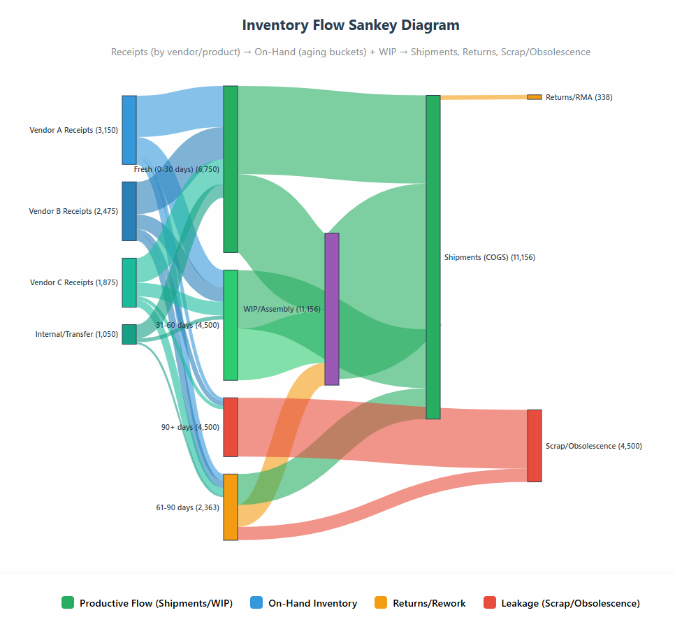
- Extending Snowball to Cash & Inventory — Apply the same flow lens to cash (AR ⇄ AP ⇄ Cash) and inventory to improve CCC, turns, and margin.
- Augmenting Financial Analysis with Agentic AI Workflows — Use agentic AI for close acceleration, probabilistic ARR forecasting with prescriptive actions, and causal variance analysis.